The Case for Scenario Coverage for Gas Detector Placement
In the beginning, gas detector placement was done by assigning detector locations based on a uniform grid in process areas where the spacing of the detectors was based on a design basis gas cloud. Typically, this was a 5 meter grid, because a 5 meter grid would always be capable of detecting a spherical gas cloud whose size could result in a vapor cloud explosion. While this approach is logical, it also results in very large, and often prohibitively expensive, numbers of gas detectors.
The next step was the use of computer software that considered 3D models of process plants, and then overlaid the “coverage” of a detector to detect that design basis 5-meter diameter clouds (which is basically a 5m radius sphere around the detector) into the model and performed a calculation of the coverage of the gas detectors by determining what portion of a covered area is inside the spheres. This is shown graphically using Kenexis Effigy FGS mapping software in the figure below.
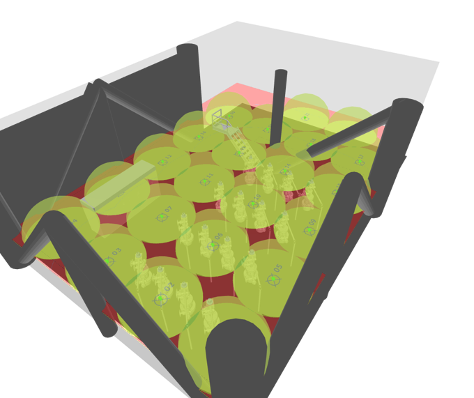
In this case the analysis was done for a typical wellbay zone for an offshore oil and gas production facility. The individual wells were analyzed for risk and assigned a Grade of B with 80% coverage, in accordance with ISA 84.00.07-2018. In order to achieve the coverage target, 22 point gas detectors were required.
While this result might have been state-of-the-art 10 years ago, technology has developed since then. This improvement in the technology for gas detector placement was driven by the fact that geographic methods result in very high detector counts that are typically questioned by management as being unreasonable, especially when they receive the price tag. Ultimately, geographic coverage does not tell you anything about how well a gas detection system will detect leaks. Geographic methods do not optimize coverage they optimize spacing. Geographic coverage does not consider the following critical factors that impact gas detection design:
- Where are releases occuring
- How big are the released gas clouds
- What effect does weather have on the released gas cloud
- Different equipment items leak at different frequencies
Geographic coverage is a geometry only exercise that does not actually consider the releases of gases and the risk that those releases pose. The Purdue Process Safety Assurance Center (P2SAC) sponsored research that showed that using geographic methods actually provides coverage that is worse than placing detectors randomly for an equal number of detectors. (https://engineering.purdue.edu/P2SAC)
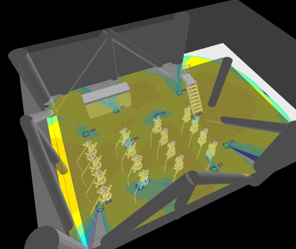
The remedy to this problem is to use scenario coverage instead of geographic coverage. When using scenario coverage, you being by running dispersion models to determine the extents of a gas cloud that could be released from equipment in the zone and then consider the release frequency based on industrial data for leak rates and hole size distribution. This data is considered in combination with local weather data related to the frequency of which the wind comes from the various different directions. Scenario coverage is the calculated by releasing the gas cloud in multiple different directions (up to 720 for Vertigo), weighting the likelihood of release in each direction by the frequency at which the wind is expected to occur in that given direction. The result is a scenario risk map, as shown below that shows, by color code, the frequency at which a gas cloud will exist in any given location.
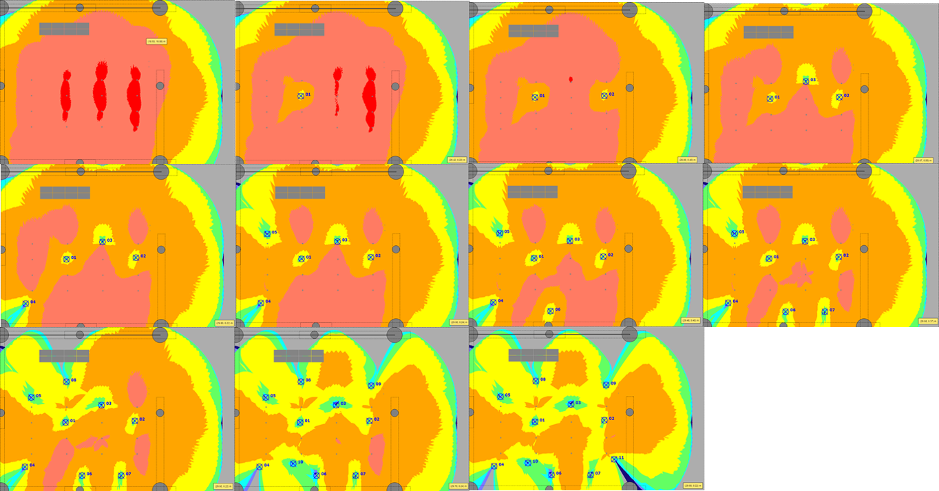
Calculation of the scenario coverage proceeds by analyzing each individual gas cloud (for this example, there were 11,520 individual clouds assessed) to determine if the cloud intersects with a detector. If so, the frequency of that added to the total frequency of all detected clouds, which is subsequently divided by the total release rate to calculate the scenario coverage. The figure below shows a series of scenario coverage maps created after the addition of individual detectors. The drawing is a plan view of residual scenario risk where all scenarios that are detected by the gas detection array are removed from the drawing and the colors shown represent the frequency of existing of gas clouds that are not detected by the gas detection array. As an analyst lays out detectors they will proceed by looking at the hottest color (red) which indicates the most frequent exposure to gas clouds and placing a detector in that location. Additional detectors are progressively added to reduce the frequency of undetected gas clouds. In the figure below you can see the progression from no detection up to in excess of 80% coverage (achieving the coverage target).

Another way to look at the effectiveness of gas detectors is by plotting the number of detectors against the scenario coverage that is achieved. In the next figure you can see that the first detector provided 13% scenario coverage. Each subsequent detector provides less, and as more and more detectors are added there are dimishing returns for additional investment in detectors.
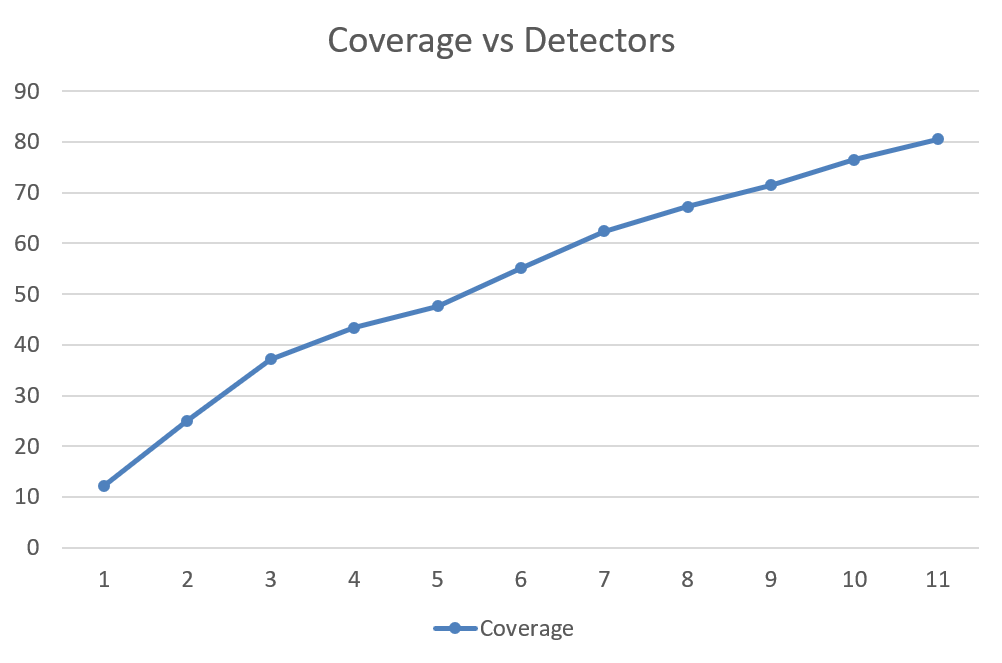
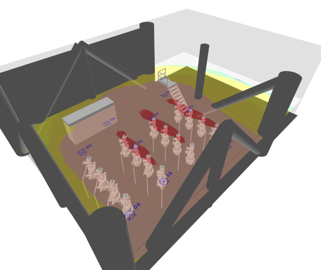
Using scenario coverage, the goal of 80% coverage was achieved with only 11 detectors instead of the 22 that were recommended by scenario coverage. This is not surprising outcome. Scenario coverage allows the focus of detector placement to be on the area where risk is highest. Scenario coverage also clearly shows where gas clouds are most likely to occur as a function of their size, as determined by dispersion modeling, and weather conditions. Furthermore, especially for high pressure systems, while a 5 meter diameter gas cloud might be able to cause harm, the actual dimensions of a gas cloud release by even a very small hole are much larger than 5 meters in diameter. This is why scenario coverage generally results in a much lower detector count all the while provide better actual coverage of releases.